
This year's busiest working day is ahead for our hero from Lapland. Delivering the presents is (in the world of optimization) a typical travelling salesman problem (TSP) - how to visit a number of locations using the shortest path available.
While the exact number of locations is hard to pinpoint, that's no reason to leave an interesting problem unsolved. We can always go for an approximate solution and change the inputs to increase understanding.
Finding the shortest route between a number of locations is no easy feat, because of the combinatorial nature of the problem. The number of possible routes to choose from is (n-1)!, which can be approximated using Stirling’s formula to:
![]()
which is probably larger than any number you’ve ever heard. Transforming to more familiar base-10 notation we get:

So in conclusion Santa has
1010 000 000 options to choose between.
Looking at that number it is pretty impressive that the current shortest solution to the problem is only 0.0471% longer than the optimal route.
The solution is that Santa would have to fly around 7 515 756km in order to visit all the cities in the world. That is a baffling 188 times around the globe or almost 10 times to the moon and back. Even putting that number into context, it feels somewhat detached from reality.
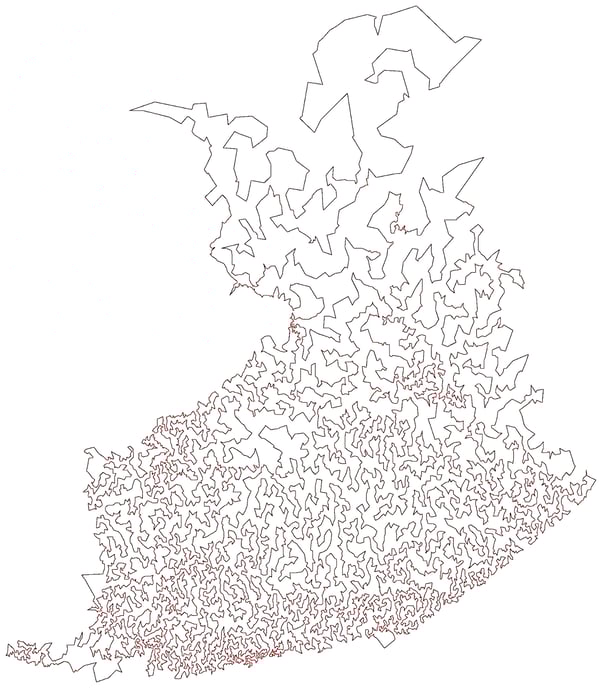
Let’s use something more ordinary like Finland. Finland is after all a pretty average country (65th in terms of size and 115th in population out of 190-ish), plus it is Santa’s home.. Using the same data source as previously, we find that there exists an optimal shortest path for visiting the 10 639 largest settlements in the country! This optimal route is merely 54 020km long.
I must however admit I would not be too happy if Santa just left my presents in the market square. Consumers are fairly demanding, and nothing short of home delivery is acceptable with regard to their Christmas presents.
So how much extra distance does the last mile delivery add to this optimal route?
I am not aware of a dataset which includes the addresses of all Finnish inhabited households. Also if there was one, I’d probably violate GDPR by using it, so let’s go with an approximate solution instead. Suppose we're operating on a flat surface and consider a square the size of 1km2. We assume further that there are n visiting locations randomly distributed on the surface and denote the shortest path visiting all of these by Ln. Interestingly enough, it's not yet known what the expected shortest path length E(Ln) is! There are however bounds for it. According to Wikipedia it’s almost surely in the following interval
![]()
So for 100 randomly scattered households in a given square kilometer Santa could expect to travel at least 7.62km and at most 15.89km. That’s quite a wide interval and looking at some computational studies, we notice that the upper bound is definitely too conservative. There is also Steinerberger (2014) showing a considerably narrower theoretical interval:
![]()
Image: Last-mile deliveries on top of the route which covers all settlements.
There are approximately 100 000 populated square kilometers in Finland, 100 338 to be exact. Average household size is 2.02, so we can divide each square's population by that number to get the number of visiting locations.
Considering that some of the inhabited squares are actually very sparsely populated, the most advisable course of action is to use the computational estimates for squares with sparse population and the theoretical bounds for the densely populated areas.
Out of these squares 96 125 have less than 100 households. Let’s use computational estimates for these and theoretical bounds for the rest (for squares with 1 household we assume within-square travel to be zero). This gives us a total route length of 210 000 - 232 000km from within-square travel.
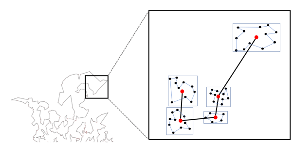
Image: Last-mile deliveries on top of the route which covers all settlements.
There is one slight issue though - 100 338 is somewhat higher than the number of settlements in our optimal route (10 639), so we have to do some hand-waving applied mathematics.
We could “squeeze” population into the 10 639 most populated squares in the data set, which would result in an underestimate of the within-square travel, because higher population density leads to more efficient last mile delivery.
We can also just add the numbers together and ignore any travel between populated squares, which isn’t covered by the original shortest route. This leads to a slight underestimate of the total route length.
On the other hand, assuming a random distribution on the populated squares is not completely realistic - settlements are usually clustered in some way, which means that we have a slight overestimate on the within-square-travel.
To summarize, the approximations partly cancel each other out and I am just going to add the numbers together.
In conclusion Santa has around 275 000km of domestic travel to expect on Christmas Eve.
Traditions in families differ, but most presents are given out between 15 and 19 o’clock. That gives an average speed of 68 750 km/h ~ 19 km/s. That is not completely out of this world - spacecraft sometimes travel faster than that. At least if Santa seems to be in a hurry, now you know why!
As a final note one word of caution. Despite the chilly weather, offering Santa a whiskey shot for warming up is definitely not recommended. If just one in ten households offers him 2cl of whiskey, already by the midpoint of his route poor Santa’s blood alcohol content is asymptotically approaching 1000 ‰.